
Scrapin' the Bizkit Part 2: Re-Arranged
I scraped some Limp Bizkit data from setlist.fm a while ago to perform some analysis. I learned a lot about the basics of scraping, some command line tools. But, I wasn’t happy with the results. I had to wait about an hour to get all the data I needed. Surely, there must be a better way.
After some research, I ditched Playwright and used some other tools to grab the info I wanted. I also tossed out the spreadsheets and used SQLite to store and query my data. Today, I’ll share my findings, and teach you everything I learned about SQLite as a result of this exercise, which was a lot.
If you’d like to follow along with my work, take a look at this branch in the GitHub repository for my scraper. Let’s talk about the improvements to the scraper first.
Improved scraping speed
Previously, I used Playwright to grab information from setlist.fm. I opened each concert page one by one to find the data I wanted to grab. But, as I noted before, I can obtain the information I need by just requesting the HTML from the concert link I needed. This meant that I did not need an entire browser to find what I’m looking for.
I demonstrated that I could request the HTML using the curl command. If you’d like, you could try it yourself, assuming curl is installed on your system.
curl https://www.setlist.fm/setlist/limp-bizkit/2024/somerset-amphitheater-somerset-wi-4ba8b3ea.html
This HTML was obtained within milliseconds; grabbing the HTML by itself instead of waiting for assets to finish loading increased speed dramatically. But since I wanted to write my script in TypeScript rather than bash, I decided to use the axios library to request the HTML using a simple interface.
let res = await axios.get(lbUrlBase + page, axiosOptions);
Now that I have the HTML I need saved into the res variable, I needed a way to parse it, preferably one that supports the HTML node querying methods to which I’ve been accustomed. jsdom was a good fit for this.
const dom = new JSDOM(res.data);
const eventList = dom.window.document.querySelectorAll(".vevent");
Compiling and running the code with swc was easy at first with just one file, like in my previous iteration. But, I ran into hiccups after attempting to separate my code into modules. I decided to let bun compile my TypeScript for me instead.
So, why didn’t I use bun to begin with? At the time of my previous writing, bun did not support some Node.js functions to create and write to files. However, those issues have been fixed with later iterations.
Once all of these pieces were put into place, I had to make some modifications to how I iterated through all the setlist.fm pages containing Limp Bizkit’s concerts. Instead of entering each concert one at a time, I gathered all the URLs that pointed to individual concert page from the search results. Once I had this array, I requested the HTML from the concert, did my parsing, and moved to the next one until I was finished.
So how much time did each of these approaches take? Here’s a table showing the time it took to scrape a single page’s worth of concerts 10 times. I used hyperfine to perform my benchmarks.
| Scraper | Mean (s) |
|---|---|
| Bun, Axios, and JSDom | 5.151 |
| Playwright | 28.324 |
That’s about five and a half times faster than before! As you can expect, these savings add up. Suppose I would like to capture concert data for 100 pages worth of concerts. With Playwright, scraping would take about 45 minutes. With bun, axios, and jsodom, scraping would take less than 10 minutes.
Instead of writing the data to a TSV file like last time, I also wanted to use a relational database to see if that was a better experience.
Improved data storage
I originally stored my scraped data into a TSV file that contained data which looked like this:
| Order | Song | Info | Concert | Date |
|---|---|---|---|---|
| … | … | … | … | … |
| 9 | Full Nelson | (with fan) | Limp Bizkit at Sonic Temple 2024 | 2024-05-19 |
| 10 | Faith | (George Michael cover) | Limp Bizkit at Sonic Temple 2024 | 2024-05-19 |
| 11 | Take a Look Around | Limp Bizkit at Sonic Temple 2024 | 2024-05-19 | |
| … | … | … | … | … |
As you can see, a lot of this data is repeated. The rows in the Concert and Date columns repeat for each performance that takes place in the same venue and day. Additionally, Song names repeat each time that song was performed. You would see the name “Nookie” over 500 times in this file in my first iteration.
This issue was remedied by using SQLite, a lightweight, relational database. With SQLite, I can create tables of data, and connect them to individual performances via an ID by using join statements. Instead of repeating the same rows of data, I can relate two groups of data by an ID, which takes up less space.
To see the space savings, I decided to test how large the TSV file and the SQLite database files would be after scraping one page, versus all the entries. Here are the results after one page.
| Scraper | Size (Kb) |
|---|---|
| TSV with Playwright | 9.8 |
| SQLite Database with Bun | 24 |
Curiously, the size of the database was almost 2.5 times larger than the TSV file. But notice the size difference once I scraped all the data with both methods.
| Scraper | Size (Kb) |
|---|---|
| TSV with Playwright | 813 |
| SQLite Database with Bun | 308 |
Now the database size is about 2.6 times smaller than the text file, even though the database contains more data than the TSV. It’s clear that using an SQLite database is more space efficient than using a TSV.
But getting the data from these files to perform analysis is wildly different. How do spreadsheet functions and SQL queries compare with each other?
Comparing queries
Last time, I used 8 pages worth of spreadsheets for filtering and analysis. The logic behind those queries started to get out of control and illegible. For instance, here’s a function that get the total number of concerts Limp Bizkit performed in the year 2023 with LibreOffice’s built-in functions.
=COUNTIFS(
  $Concerts.$A$2:$B$769 , ">="&DATE($A209,1,1),
  $Concerts.$A$2:$B$769, "<"&DATE($A208,1,1)
)
COUNTIFSis a function that increments a count if a certain condition is satisfied.- Odd numbered parameters (the first and third in this case) are the ranges of data to consider.
- Even numbered parameters are the conditions that must pass to increment the counter.
">="&DATE($A209,1,1)is a condition that says “greater than or equal to the date at year$A209, month 1, and day 1,” or January 1st,$A209$A209is the value in the cell of columnA, row209
- The second condition says any dates less than January 1st,
$A208.
If $A208 is 2024, and $A209 is 2023, then this function will return the number of concerts within 2023. That is, if the $Concerts sheet contains the expected information.
In fact, this command is very brittle. If the data in the $Concerts sheet changes for whatever reason, or the data from the A column where the years are located changes, the calculation is thrown off!
Compare this to the equivalent query in SQL.
select count(*) as "Number of concerts" from concerts
where strftime("%Y", date) = "2023";
selectis the statement that says “give me this data.”count(*)is a function that returns the number of all the rows in a query.fromindicates where I want to get this data. In this case, I want to get this info from theconcertsdatabase.wherefilters out the data I receive that passes certain conditions. In this case, I’m only selecting rows that have a year of2023.
Whichever you like more is a matter of opinion, but this SQL query reads a little more like natural language compared to the spreadsheet function above.
But what if I wanted the number of concerts performed in every year since 2000? It’s trivial to copy and paste the function into the following rows, assuming you have a column of years iterating from 2024 to 2000. In the spreadsheet, the function is (almost) copied for each year in an adjacent column, like so:
| Year | Number of concerts query |
|---|---|
| 2024 | =COUNTIFS($Concerts.$A$2:$Concerts.$B$769 , ">="&DATE($A208,1,1)) |
| 2023 | =COUNTIFS($Concerts.$A$2:$Concerts.$B$769 , ">="&DATE($A209,1,1), $Concerts.$A$2:$Concerts.$B$769, "<"&DATE($A208,1,1)) |
| 2022 | =COUNTIFS($Concerts.$A$2:$Concerts.$B$769 , ">="&DATE($A210,1,1), $Concerts.$A$2:$Concerts.$B$769, "<"&DATE($A209,1,1)) |
| … | … |
That’s a lot of noise, but fortunately most spreadsheet software will automatically handle incrementing indexes that are not prepended with a $. To get this information with SQLite, we can try this.
select
  strftime("%Y", date) as year,
  count(*) as count
from concerts
where year >= "2000"
group by year
order by year desc;
group bygroups all the rows together by year. Once the rows are grouped together, thencount(*)will count the number of rows per group.order byorders the data by a given column.descindicates the data should be descending.
Note this is almost the same as the data from my spreadsheets. The only thing that’s missing are years when there are zero concerts. They are skipped in the SQL query above. To get all the years including ones that have no concerts, you would need to do additional work. It’s challenging to iterate over a series of values with SQLite.
Whatever your needs are, spreadsheets and databases can be useful. However, my intuition is that SQL is a hotter skill than spreadsheets, and a quick LinkedIn search seems to agree.
| Skill | Number of job search results |
|---|---|
| SQL | 426,766 |
| Spreadsheets | 69,254 |
This is the part where I talk a lot about SQL. I’ll go through the steps I took to organize and query my data. First, let’s talk about the tables.
Want to try these queries yourself?
If you’d like to try some of these commands yourself, I recommend installing sqlite3, and using it to open the lb.db database file within my repository like so:
# assuming you're in the root of the lb-scraper directory
sqlite3 data/lb.db
Try running the .tables command once you’re within the SQLite shell. If your output looks like this, then you should be good!
sqlite> .tables
concerts                           performances
fan_performances                   performances_view
fan_performances_small             performances_view_small
fan_performances_with_instruments  songs
Alternatively, you can use a GUI such as DB Browser for SQLite to view the data. Type the queries in the “Query” tab and click the run button to give them a try!
Intro to SQL
The data schema
I’ll be using the following definitions in this project:
- A performance is the performing of one song at one concert. It also has an order in which the performance occurs in the show.
- A concert is a collection of performances on a day and location
- A song is a song that is performed at a concert. This song can be performed multiple times across multiple concerts.
I defined these SQL tables to represent this data. Here are the concerts.
create table concerts(
  concertId integer not null primary key,
  date string not null, -- YYYY-MM-DD
  venue string not null
);
- The
concertIdis important because it distinguishes rows of data from one another, and will later be used to connect tables together to view data easily. - Note that comments in SQL start with
--. These comments persist when the table is created, which serves as nice documentation not nullguarantees I don’t accidentally create a concert without adateor avenue.
Next comes the songs.
create table songs(
  songId integer not null primary key,
  name varchar not null unique
);
- I don’t want multiple rows of songs to have the same
name, so I use theuniquekeyword here.
Finally, the most important table, the performances. Notice the foreign key declarations in the schema below.
create table performances(
  performanceId integer not null primary key,
  notes varchar, -- performance notes (optional)
  songOrder integer not null, -- order in which the song was played
  concertId integer not null,
  songId integer not null,
  foreign key (concertId) references concerts(concertId),
  foreign key (songId) references songs(songId)
);
The foreign key command creates a relationship between performances and concert tables, and performances and song tables. A performance contains references to one song and one concert. Take a look at this line below:
concertId integer not null,
--- ...
foreign key (concertId) references concerts(concertId)
The concertId of the performance references the concertId of a concert in the concerts table. And because the concertId in a performance cannot be null, I need to know the concert the performance takes place before I can create a new performance in the database. I also need to know the song as well.
Foreign keys are the key to the increased storage efficiency mentioned above. By only saving IDs for songs and concerts in the performances table, I no longer need to duplicate song names and venues across thousands of performances.
Let’s see how we can query the data to get the same information from my old TSV.
Creating an SQL query
As a reminder, my TSV with performance data used to have columns that looked like this:
| Order | Song | Info | Concert | Date |
|---|
However, my columns in my performances table looks like this:
| performanceId | notes | songOrder | concertId | songId |
|---|
How can I coerce the data I’ve collected into a format that is similar to the TSV? First, let’s create a query that gets the data we want. We’ll start with selecting the columns.
select
  songOrder as "Order",
  songs.name as Song,
  notes as Info,
  concerts.venue as Concert,
  concerts.date as Date
- You’ll notice some columns refer to our
songsandconcertsdatabase, such assongs.nameandconcerts.venue. This queries the column that belongs in those respective databases, which we’ll address soon.
Why do I need quotes around "Order"?
Order is an SQL command, and, in case you haven’t noticed, SQL is case-insensitive. The quotes specify that "Order" is a label I would like to use, and not the command itself.
If I didn’t have the quotes around Order, my query would break with the following error:
Error: in prepare, near "Order": syntax error (1)
Next, we’ll indicate where we’ll get the columns from, like so:
from performances
songOrderandnotesare obtained straight from theperformancesdatabase
But what about the Song, Concert, and Date columns? To share data from the other databases, we’ll use a join statement. With this, we can add data from other tables to the row that matches a certain condition. Below, we’ll add concert data from the concerts table when there’s a match between the concertId in the performances table.
join concerts on performances.concertId = concerts.concertId
As a shortcut, you can use the using clause in your join statement if the columns you’re connecting have the same name. We’ll add the songs here too, since the command is similar. Don’t forget the parentheses around the column names!
join concerts using (concertId)
join songs using (songId)
All in all, here’s the entire query that matches the layout of the old TSV file.
select
  songOrder as "Order",
  songs.name as Song,
  notes as Info,
  concerts.venue as Concert,
  concerts.date as Date
from performances
join concerts using (concertId)
join songs using (songId);
And you can see it’s output below.
| Order | Song | Info | Concert | Date |
|---|---|---|---|---|
| 1 | Break Stuff | Ruoff Music Center, Noblesville, IN, USA | 2024-07-21 | |
| 2 | Just Like This | (Tour debut) | Ruoff Music Center, Noblesville, IN, USA | 2024-07-21 |
| 3 | Hot Dog | Ruoff Music Center, Noblesville, IN, USA | 2024-07-21 | |
| 4 | My Generation | Ruoff Music Center, Noblesville, IN, USA | 2024-07-21 | |
| 5 | Rollin’ (Air Raid Vehicle) | Ruoff Music Center, Noblesville, IN, USA | 2024-07-21 | |
| … | … | … | … | … |
Creating SQL views
The above query is useful, but we don’t want to have to type this entire query each time we want to work on this data. Much like how you can save variables when writing code, you can create an SQL view to save a query for later use.
Creating a view is simple. Let’s make a view using the previous query called performances_view.
create view performances_view as
select
  songOrder as "Order",
  songs.name as Song,
  -- The rest of the command
Once created, you can use the view in select queries like you would with any SQL table!
select * from performances_view;
Remember when I was manipulating my old data with command line tools to sort and filter my output? That was pretty cool, but SQL allows me to perform these actions within the database itself, and I can save those queries into their own views. This will make comparing performances with and without fans much simpler.
First, we’ll create a view that filters the performances by fan interactions.
create view fan_performances as
select * from performances_view
where lower(notes) like "%fan%" or
lower(notes) like "%audience%" or
lower(notes) like "%crowd%" or
lower(notes) like "%guest%";
whereis a statement that only returns rows which match a condition.lower()is a function that converts all characters in a string to lower case. This prevents me from having to distinguish betweenfanandFanin my search.likeis a statement that searches for a specific pattern in a string. The format string uses the%wildcard, which matches zero, one, or multiple characters. So,%fan%matches any rows wherefanappears anywhere in the string.oris used to match any of the cases that are present in thewherestatement. I’m looking for notes that contain the wordsfan, oraudience, orcrowd, orguest.
Now that we have fan_performances, let’s filter even further with fan performances that contain instruments.
CREATE VIEW fan_performances_with_instruments as
select * from fan_performances
where lower(notes) like "%guitar%" or
lower(notes) like "%bass%" or
lower(notes) like "%band%" or
lower(notes) like "%instrument%"
At this point, we’ve saved our data to a database, and we’ve created some virtual tables to simplify our database queries. If we want to have more robust queries, however, I should first explain what CTEs, or Common Table Expressions are.
Common Table Expressions (CTEs)
CTEs are used to compose queries together. The output of one query can be represented as its own table, which can then be fed into another query. Here’s an example that uses a CTE to create a temporary view called song_counts, and queries the first 10 results.
-- This is the Common Table Expression
with song_counts as (
  select songName as name, count(*) as count from performances_view group by songName order by count desc
)
-- we can now reference song_counts in our query below
select count, name from song_counts
limit 10;
withassigns the CTE to a name. The query within the parentheses will be assigned to the namesong_counts
Although getting the top 10 songs performed in concerts can be done without a CTE, this demonstrates the concept, which will be important for the analysis below. If there are any other new concepts that appear, I’ll explain them below the relevant tables.
With this in place, we’re ready to analyze the data. Let’s see some plots and charts!
Data analysis with SQL
Likelihood of fan interaction
In my previous article, I learned that the ratio between performances with fans and band performances was abysmally small. About 1.6% of performances have fan interaction.
-- Fan performances count
with fpc as (
  select count(*) as count from fan_performances
),
-- Total performances count
tpc as (
  select count(*) as count from performances
)
select
  'with fans' as "Performances",
  fpc.count as "Number of performances"
from fpc
union
select
  'without fans' as "Performances",
  (tpc.count - fpc.count) as "Number of performances"
from fpc, tpc
union
select
  'total' as "Performances",
  tpc.count as "Number of performances"
from tpc
order by "Number of performances";
unionsits in between twoselectclauses. This means that data from theseselectclauses will be put together in the table. This is done to combine the three rows with the labels ‘with fans’, ‘without fans’, and ‘total’ together.- You may see
union all, which is similar tounion, except rows with duplicate data is permitted.
- You may see
| Performances | Number of performances |
|---|---|
| with fans | 164 |
| without fans | 10290 |
| total | 10454 |
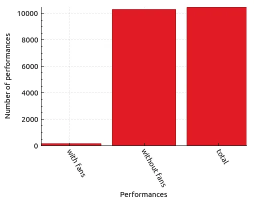
This paints a very bleak picture. Most performances do not have some sort of fan interaction. However, it’s not expected that fans will be on stage for every song performance in each concert. Let’s zoom out a little bit and compare the number of concerts with fan interaction compared to the total number of concerts.
First, let’s get all the concerts with fan performances.
with fan_concerts as (
  select venue from fan_performances group by venue
)
select count(*) from fan_concerts;
-- 116
You can use a CTE in place of a table without using the with expression, so the line above can be rewritten to this:
select count(*) as count from (
  select venue from fan_performances group by venue
)
-- still 116!
Then, we’ll get the total number of concerts.
select count(*) from concerts;
-- 846
Now that we have these tables, we can use our expressions in our query below. Note how similar this looks to the number of performances query above with its unions.
with fan_concerts as (
  select count(*) as count from (
    select venue from fan_performances group by venue
  )
),
total_concerts as (
  select count(*) as count from concerts
)
select
  'with fans' as "Concerts",
  fc.count as "Number of concerts"
from fan_concerts fc
union
select
  'without fans' as "Concerts",
  (tc.count - fc.count) as "Number of concerts"
from fan_concerts fc, total_concerts tc
union
select
  'total' as "Concerts",
  tc.count as "Number of concerts"
from total_concerts tc
order by "Number of concerts";
| Concerts | Number of performances |
|---|---|
| total | 846 |
| with fans | 116 |
| without fans | 730 |
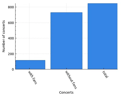
This means that 13.7% have some level of fan interaction according to this data. There a little more than a 1 in 10 chance Limp Bizkit will interact with fans if you were equally likely to go to any of their shows at any point in their career.
However, I’m not a time traveler, so let’s focus our look for during their current tour. The Loserville Tour started on July 16th, 2024, so to modify the queries to only search for concerts since then, we’ll do the following.
with fan_concerts as (
  select count(*) as count from (
    select venue from fan_performances
    where date >= "2024-07-16"
    group by venue
  )
),
total_concerts as (
  select count(*) as count from concerts
  where date >= "2024-07-16"
)
-- ...
| Concerts during Loserville tour | Number of concerts |
|---|---|
| with fans | 4 |
| without fans | 5 |
| total | 9 |
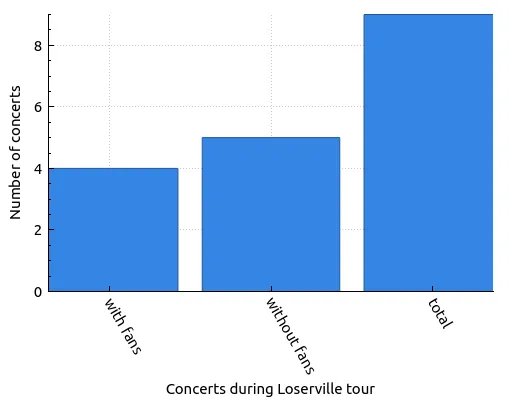
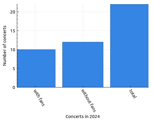
So, according to data from their current tour, there’s about a 45% chance that Limp Bizkit will interact with fans in some exciting way, like inviting fans on stage to perform. Interestingly enough, this trend has been pretty consistent since the beginning of 2024! Modifying the query to search from January 1st yields these results:
| Concerts in 2024 | Number of concerts |
|---|---|
| with fans | 10 |
| without fans | 12 |
| total | 22 |
Number of fan performances with instruments
We used the total number of fan performances with instruments to decide which songs we should practice in the off chance we make it on stage to play. Our original data from the spreadsheet looked like this:
| Song | Count |
|---|---|
| My Way | 5 |
| Hot Dog | 4 |
| Eat You Alive | 2 |
| Gold Cobra | 1 |
| Take a Look Around | 1 |
| Pollution | 1 |
| My Generation | 1 |
We can compare our newly scraped data with our previous findings by using this SQL query below.
select
  songName as "Song",
  count(*) as Count
from fan_performances_with_instruments
group by songName
order by Count desc;
| Song | Count |
|---|---|
| My Way | 5 |
| Hot Dog | 4 |
| Eat You Alive | 2 |
| Take a Look Around | 1 |
| Pollution | 1 |
| My Generation | 1 |
| Gold Cobra | 1 |
| Faith | 1 |
| Break Stuff | 1 |
| 9 Teen 90 Nine | 1 |
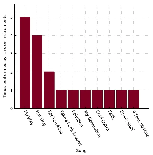
There are a few additional entries in this list! Have there been some new fan performances on instruments? Let’s check.
select date, songName, notes
from fan_performances_with_instruments
where date > "2024-01-01"
order by date desc;
-- |date|songName|notes|
-- |2024-07-24|Break Stuff|(All opening bands + some fans on stage)|
-- |2024-06-22|Faith|(George Michael cover)(With Gabriel, young guitarist from the crowd)|
It appears that one performance qualifies! Gabriel, a fan, can be seen playing in this video of this performance of Faith here! But according to the video evidence of the Break Stuff performance, fans get on stage, but none of them have a mic, or are playing an instrument. Therefore, it’s not a performance.
We can edit the data within this row by going back to the source. Let’s find the performance that contains the relevant notes.
select * from performances
where notes like "(All opening bands + some fans on stage)";
-- 10440|(All opening bands + some fans on stage)|17|844|1
The performanceId of this row is 10440, so we’ll use the update and set statements to modify this row’s notes.
update performances
set notes = "(All opening acts + some fans on stage)"
where performanceId = 10440;
Now we double-check if our changes went through as expected by selecting the same row and reviewing its output.
select * from performances where performanceId = 10440;
-- 10440|(All opening acts + some fans on stage)|17|844|1
Now let’s check our previous instrument performance query to see if our data is as expected. Remember, we should see “Faith” appear in our bar chart.
| Song | Count |
|---|---|
| My Way | 5 |
| Hot Dog | 4 |
| Eat You Alive | 2 |
| Take a Look Around | 1 |
| Pollution | 1 |
| My Generation | 1 |
| Gold Cobra | 1 |
| Faith | 1 |
| 9 Teen 90 Nine | 1 |
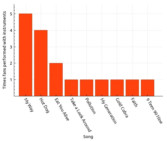
Everything looks good! By our count, the choices we made for songs to learn are still pretty good. But is there more we can learn about the songs that we’ve picked? Are they even being played in this tour?
The likelihood X song will be performed during Loserville?
We can view this question in two parts. First, let’s determine the likelihood a song will appear on this tour at all. To do this, we’ll need to following information:
- The number of concerts in which a song was performed
- The number of concerts that has occurred since the start of Loserville (July 16th, 2024)
Dividing these two numbers will give us the percentage of concerts that song has appeared.
Let’s first start with the number of concerts, since that’s pretty straightforward.
select count(*) from concerts where date >= "2024-07-16";
-- 9
Now, using our performances_view from before, let’s find all times that “My Way” was performed.
select songName, count(distinct date) as Count
from performances_view
where date >= '2024-07-16'
and songName is "My Way";
distinctis used in thecountfunction to specify I should only count unique, non-null values from thedatecolumn in theperformances_view. This will cover the case where there are encores of the same song in one concert, since that’s not relevant to the number of concerts in which “My Way” was played
Combining the two queries from above, we can find the percentage of time “My Way” was performed
with performances_count as (
  select songName, count(distinct date) as Count
  from performances_view
  where date >= '2024-07-16'
  and songName is "My Way"
),
total_concerts as (
  select count(*) as total from concerts where date >= '2024-07-16'
)
select
  "My Way" as SongName,
  coalesce(pc.Count, 0) as Count,
  tc.total as Total,
  round(cast(Count as float) / cast(Total as float) * 100.0) as Percentage
from performances_count pc
join total_concerts tc;
coalesceis often used for replacingnullvalues. Ifpc.Countisnull(which may happen if a song has not been played during Loserville, in this case), then the value in this row will be the second parameter,0.roundrounds the result of its input to the nearest digit.castallows you to convert a value from one type to another. In SQL, integer division rounds the quotient to the nearest digit (select 1 / 9;returns0instead of0.111..., for example). To get thePercentagevalue, theCountandTotalvalues must be cast as floating point numbers.
| SongName | Count | Total | Percentage |
|---|---|---|---|
| My Way | 9 | 9 | 100.0 |
The table confirms that “My Way” has been performed in 100% of the concerts during the Loserville tour. It would be nice to compare the percentages of “My Way,” “Hot Dog,” and “9 Teen 90 Nine” together. How do we use this same query for a range of values?
Let’s first create a table that contains a column of our three song names.
select "My Way" as Song
union
select "Hot Dog"
union
select "9 Teen 90 Nine";
- Remember
union? All the rows in theseselectswill be combined into one table. I specify the column name in the firstselectstatement, otherwise the column name would be called"My Way", which is confusing.
| Song |
|---|
| 9 Teen 90 Nine |
| Hot Dog |
| My Way |
Now that I have the table with the songs I want, I can combine them with my previous queries to get the table of percentages that I want. This query below gets the percentage of concerts that these songs appear in during the Loserville tour.
with Songs AS (
  select 'My Way' AS Song
  union all
  select 'Hot Dog'
  union all
  select '9 Teen 90 Nine'
),
performance_counts AS (
  select songName, count(distinct date) as Count
  from performances_view
  where date >= '2024-07-16'
  and songName in (select Song from Songs)
  group by songName
),
total_concerts AS (
  select count(*) as total from concerts where date >= '2024-07-16'
)
select
  s.Song,
  coalesce(pc.Count, 0) as Count,
  tc.total as Total,
  round(cast(Count as float) / cast(Total as float) * 100.0) as "Percentage of concerts"
from Songs s
left join performance_counts pc ON s.Song = pc.songName
join total_concerts tc
order by s.Song;
- The
inkeyword is used withwhereto match a row with a series of values. In this case, if asongNamematches any of the rows from theSongstable above, then it’s included. - Notice the
performance_countstable needs to be grouped bysongName. This will ensure all of our expected songs appear in the table. - We’re joining the
Songstable with theperformance_countstable, but what if one of our songs has not been performed during Loserville? Theleft joinstatement ensures our rows in theSongstable are included in our output, even if there’s no corresponding data from theperformance_countstable. If that’s the case,nullwill appear in theCountcolumn, which will be converted to0by thecoalescefunction.
Here are the results of the query above:
| Song | Count | Total | Percentage of concerts |
|---|---|---|---|
| 9 Teen 90 Nine | 1 | 9 | 11.0 |
| Hot Dog | 9 | 9 | 100.0 |
| My Way | 9 | 9 | 100.0 |
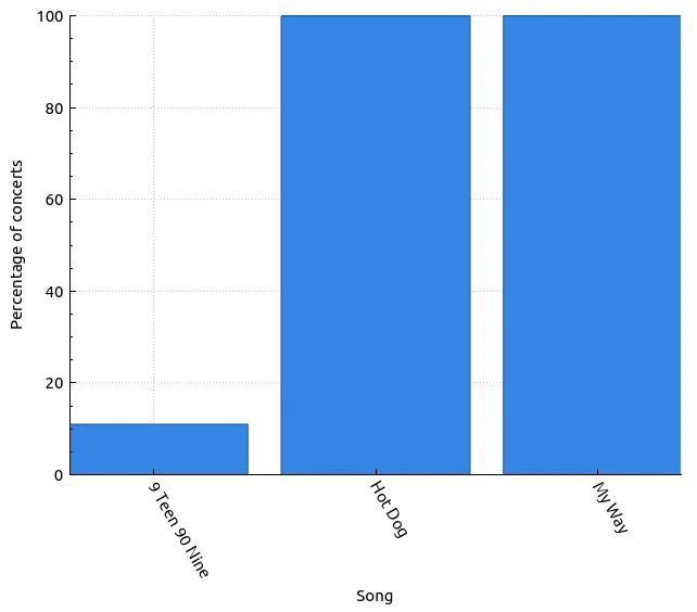
This tells us that it’s highly likely that My Way and Hot Dog will be played at the upcoming concert. This could either help or harm us, depending on when they typically play those songs. If Limp Bizkit plays our choice of song before we have a chance to get on stage, that eliminates it from our choices to play.
However, it’s encouraging to see that 9 Teen 90 Nine was played during this tour at all. We now know the band is prepared for that song, which means it’s possible for us to play it. Since the band is not likely to perform the song themselves, this gives us the opportunity to play the song in their stead.
When will X song be performed in a concert?
Let’s figure out at what point My Way and Hot Dog are played during a concert in this current tour. We’ll need the following pieces of data for each of the concerts in this tour.
- The order in which our song of choice is performed. We already have this with the
songOrdercolumn. - The total number of songs performed per concert. This is something we can calculate.
With these two values, we can create a ratio that will tell us at what point in the concert we should start making our way to the front. I called this a timing ratio last time. A timing ratio of 0 means the very beginning of the concert, while a timing ratio of 1 means the very last song.
First, let’s get the orders when “My Way” was performed.
select
  date,
  songOrder as MyWayOrder
from performances_view
where date >= "2024-07-16"
and songName is "My Way"
order by date;
| date | MyWayOrder |
|---|---|
| 2024-07-16 | 10 |
| 2024-07-18 | 6 |
| 2024-07-20 | 7 |
| 2024-07-21 | 6 |
| 2024-07-23 | 6 |
| 2024-07-24 | 9 |
| 2024-07-26 | 8 |
| 2024-07-28 | 9 |
| 2024-07-30 | 6 |
The same can be done with for “Hot Dog” like this.
select
  date,
  songOrder as HotDogOrder
from performances_view
where date >= "2024-07-16"
and songName is "Hot Dog"
order by date;
| date | HotDogOrder |
|---|---|
| 2024-07-16 | 4 |
| 2024-07-18 | 3 |
| 2024-07-20 | 2 |
| 2024-07-21 | 3 |
| 2024-07-23 | 2 |
| 2024-07-24 | 5 |
| 2024-07-26 | 4 |
| 2024-07-28 | 5 |
| 2024-07-30 | 3 |
Let’s put these two tables together with a join and see what that looks like. We’ll also add a table for 9 Teen 90 Nine, just for completeness.
select
  date,
  pv.songOrder as MyWayOrder,
  hdo.HotDogOrder as HotDogOrder,
  ndo.NineTeenOrder as NineTeenOrder
from performances_view pv
left join (
  -- Order of performances of Hot Dog
  select
    date,
    songOrder as HotDogOrder
  from performances_view
  where date >= "2024-07-16"
  and songName is "Hot Dog"
) hdo using (date)
left join (
  -- Order of performances of 9 Teen 90 Nine
  select
    date,
    songOrder as "NineTeenOrder"
  from performances_view
  where date >= "2024-07-16"
  and songName is "9 Teen 90 Nine"
) ndo using (date)
where date >= "2024-07-16"
and songName is "My Way"
order by date;
- Note that I didn’t
coalescethe value ofNineTeenOrder. In the plot below, you’ll (maybe) see the dot that corresponds to the single performance of 9 Teen 90 Nine. In this column,nullvalues are ok here.
| date | MyWayOrder | HotDogOrder | NineTeenOrder |
|---|---|---|---|
| 2024-07-16 | 10 | 4 | |
| 2024-07-18 | 6 | 3 | |
| 2024-07-20 | 7 | 2 | |
| 2024-07-21 | 6 | 3 | |
| 2024-07-23 | 6 | 2 | |
| 2024-07-24 | 9 | 5 | 4 |
| 2024-07-26 | 8 | 4 | |
| 2024-07-28 | 9 | 5 | |
| 2024-07-30 | 6 | 3 |
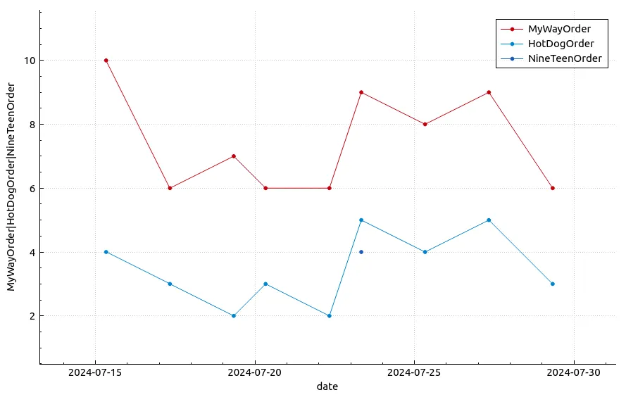
Although this doesn’t answer our questions yet, it’s interesting to see that Hot Dog typically appears earlier in the concert, which means, based on our observations about when fan performances with instruments usually take place, My Way is a better candidate to get on stage and play than Hot Dog.
To know for sure, though, we’ll need to know the timing ratio of each of these performances. Let’s keep going and figure that out. Returning to “My Way”, we can find the timing ratio for all the concerts in the Loserville tour like so.
-- rows of dates and the number of songs that were performed on those dates
with spc as (
  select date, count(*) as songsPerConcert
  from performances_view
  where date >= "2024-07-16"
  group by date
)
select
  date,
  round(cast(songOrder as float) / cast(songsPerConcert as float), 2)
    as MyWayTimingRatio
from performances_view
left join spc using (date)
where date >= "2024-07-16"
and songName = "My Way"
group by date;
| date | MyWayTimingRatio |
|---|---|
| 2024-07-16 | 0.67 |
| 2024-07-18 | 0.38 |
| 2024-07-20 | 0.39 |
| 2024-07-21 | 0.38 |
| 2024-07-23 | 0.43 |
| 2024-07-24 | 0.53 |
| 2024-07-26 | 0.53 |
| 2024-07-28 | 0.53 |
| 2024-07-30 | 0.4 |
Let’s modify the query by selecting more than one songName.
-- rows of dates and the number of songs that were performed on those dates
with spc as (
  select date, count(*) as songsPerConcert
  from performances_view
  where date >= "2024-07-16"
  group by date
)
select
  date,
  songName,
  round(cast(songOrder as float) / cast(songsPerConcert as float), 2)
    as songTimingRatio
from performances_view
left join spc using (date)
where date >= "2024-07-16"
and songName in ( "My Way", "Hot Dog", "9 Teen 90 Nine", "Full Nelson");
| date | songName | songTimingRatio |
|---|---|---|
| 2024-07-21 | Hot Dog | 0.19 |
| 2024-07-21 | My Way | 0.38 |
| 2024-07-21 | Full Nelson | 0.63 |
| 2024-07-20 | Hot Dog | 0.11 |
| 2024-07-20 | My Way | 0.39 |
| 2024-07-20 | Full Nelson | 0.67 |
| 2024-07-18 | Hot Dog | 0.19 |
| 2024-07-18 | My Way | 0.38 |
| 2024-07-18 | Full Nelson | 0.81 |
| 2024-07-16 | Hot Dog | 0.27 |
| 2024-07-16 | My Way | 0.67 |
| 2024-07-16 | Full Nelson | 0.8 |
| 2024-07-28 | Hot Dog | 0.29 |
| 2024-07-28 | My Way | 0.53 |
| 2024-07-28 | Full Nelson | 0.76 |
| 2024-07-26 | Hot Dog | 0.27 |
| 2024-07-26 | My Way | 0.53 |
| 2024-07-26 | Full Nelson | 0.73 |
| 2024-07-24 | 9 Teen 90 Nine | 0.24 |
| 2024-07-24 | Hot Dog | 0.29 |
| 2024-07-24 | My Way | 0.53 |
| 2024-07-24 | Full Nelson | 0.65 |
| 2024-07-23 | Hot Dog | 0.14 |
| 2024-07-23 | My Way | 0.43 |
| 2024-07-23 | Full Nelson | 0.86 |
| 2024-07-30 | Hot Dog | 0.2 |
| 2024-07-30 | My Way | 0.4 |
| 2024-07-30 | Full Nelson | 0.67 |
Now this next part requires some breakdown to figure out if you’re new to SQL (like I am). If we want to plot our songTimingRatios for each of our songs, we have to separate them out into their own columns. That’s the expected format our plotting software requires.
If you tried to take this table above and plot it, then here’s what would happen.
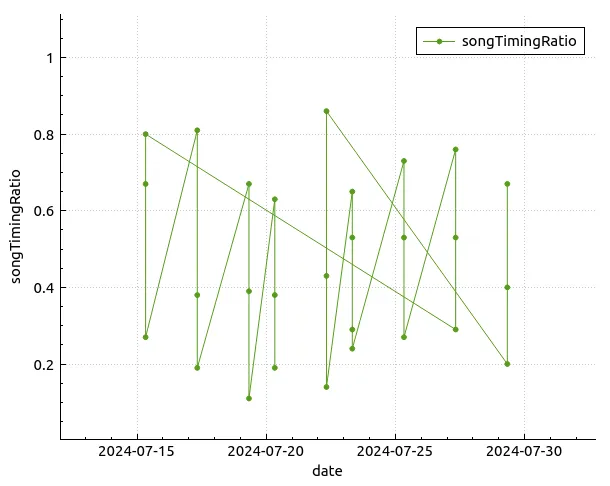
As you can see, not very helpful. Let’s move the second query from above into its own CTE to get started.
with spc as (
  select date, count(*) as songsPerConcert
  from performances_view
  where date >= "2024-07-16"
  group by date
),
-- The new CTE
songTimingRatios as (
  select
    date,
    songName,
    round(cast(songOrder as float) / cast(songsPerConcert as float), 2)
      as songTimingRatio
  from performances_view
  left join spc using (date)
  where date >= "2024-07-16"
  and songName in ( "My Way", "Hot Dog", "9 Teen 90 Nine", "Full Nelson")
)
select * from songTimingRatios;
The output is the same as the table above, which is good! This will be our base for separating each song’s timing ratios into their own column. So, how do we get the timing ratios for the song “My Way?” We can simply use a where statement to match the right song.
with spc as (
  select date, count(*) as songsPerConcert
  from performances_view
  where date >= "2024-07-16"
  group by date
),
songTimingRatios as (
  select
    date,
    songName,
    round(cast(songOrder as float) / cast(songsPerConcert as float), 2)
      as songTimingRatio
  from performances_view
  left join spc using (date)
  where date >= "2024-07-16"
  and songName in ( "My Way", "Hot Dog", "9 Teen 90 Nine", "Full Nelson")
)
select
 date,
 songTimingRatio as MyWayTimingRatios
from songTimingRatios as MyWay
where songName is "My Way"
order by date;
- I split the columns into their own entries to rename the column accordingly
- I also added an alias to indicate I’m using this table for “My Way.” This will be useful later.
As a result, our table now contains a column of timing ratios for “My Way,” like above. This table is indexed by the date.
Let’s now think of the join statement for a second. A join combines a column of data to the table when a certain condition is met. Usually, we join two tables on some kind of shared ID, but this condition can be anything we want. What if we joined the data from the songTimingsRatio table to itself given the right conditions?
What do I mean by this? Let’s take a look at the songTimingsRatio CTE.
| date | songName | songTimingRatio |
|---|---|---|
| 2024-07-21 | Hot Dog | 0.19 |
| 2024-07-21 | My Way | 0.38 |
In the query above, we get the following row:
| date | MyWayTimingRatios |
|---|---|
| 2024-07-21 | 0.38 |
Now we’d like to join this query result above with the songTimingsRatio table above when the date for both rows match and the songName is “Hot Dog.” The end result will look like this!
| date | MyWayTimingRatios | songTimingRatio |
|---|---|---|
| 2024-07-21 | 0.38 | 0.19 |
Let’s write this out.
--- CTEs from above...
select
  MyWay.date as Date,
  MyWay.songTimingRatio as MyWayTimingRatios,
  HotDog.songTimingRatio as HotDogTimingRatios
from songTimingRatios MyWay
left join songTimingRatios HotDog
  on MyWay.date = HotDog.date and HotDog.songName = "Hot Dog"
where MyWay.songName is "My Way"
order by MyWay.date;
- Notice the aliases I added in my new query to distinguish between the
MyWaytable and theHotDogtable.
This combines our column of timing ratios to our table! Success!
| Date | MyWayTimingRatios | HotDogTimingRatios |
|---|---|---|
| 2024-07-16 | 0.67 | 0.27 |
| 2024-07-18 | 0.38 | 0.19 |
| 2024-07-20 | 0.39 | 0.11 |
| 2024-07-21 | 0.38 | 0.19 |
| 2024-07-23 | 0.43 | 0.14 |
| 2024-07-24 | 0.53 | 0.29 |
| 2024-07-26 | 0.53 | 0.27 |
| 2024-07-28 | 0.53 | 0.29 |
| 2024-07-30 | 0.4 | 0.2 |
We can now use this query to plot some data! First, let’s add our timing ratios for “9 Teen 90 Nine”, and “Full Nelson.”
Why bring up Full Nelson now?
Recall that Full Nelson has the most fan participation out of all of Limp Bizkit’s songs.
select
  songName as Song,
  count(*) as "Times fans performed"
from fan_performances
group by songName
order by "Times fans performed" desc
limit 10;
| Song | Times fans performed |
|---|---|
| Full Nelson | 32 |
| Faith | 14 |
| Break Stuff | 13 |
| My Way | 11 |
| Livin’ It Up | 11 |
| Hot Dog | 11 |
| Eat You Alive | 11 |
| Rollin’ (Air Raid Vehicle) | 6 |
| Stuck | 5 |
| Nookie | 5 |
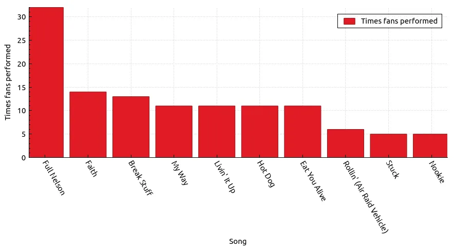
In fact 1 in 3 performances of Full Nelson have included fans from the crowd in this tour alone!
with total_full_nelsons as (
  select "Total Full Nelsons" as label, count(*) as count
  from performances_view
  where date >= "2024-07-16"
  and songName = "Full Nelson"
)
select "Full Nelsons with fans" as label, count(*) as count
from fan_performances fp
where date >= "2024-07-16"
and songName = "Full Nelson"
union
select * from total_full_nelsons;
| label | count |
|---|---|
| Full Nelsons with fans | 3 |
| Total Full Nelsons | 9 |
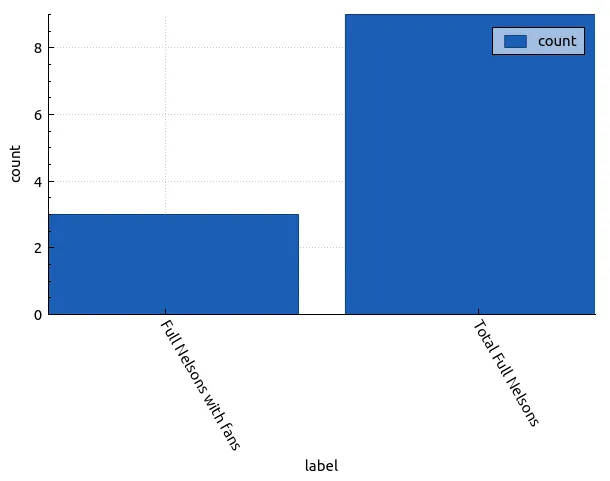
This makes Full Nelson useful to get a feel for when fan interaction will take place in a concert during this tour.
--- CTEs from above...
select
  MyWay.date as Date,
  MyWay.songTimingRatio as MyWayTimingRatios,
  HotDog.songTimingRatio as HotDogTimingRatios,
  NinetyNine.songTimingRatio as NinetyNineTimingRatios,
  FullNelson.songTimingRatio as FullNelsonTimingRatios
from songTimingRatios MyWay
left join songTimingRatios HotDog
  on MyWay.date = HotDog.date and HotDog.songName = "Hot Dog"
left join songTimingRatios NinetyNine
  on MyWay.date = NinetyNine.date and NinetyNine.songName = "9 Teen 90 Nine"
left join songTimingRatios FullNelson
  on MyWay.date = FullNelson.date and FullNelson.songName = "Full Nelson"
where MyWay.songName is "My Way"
order by MyWay.date;
And now we have the complete data set to figure out the timing during concerts when specific songs will take place. Here’s the chart below.
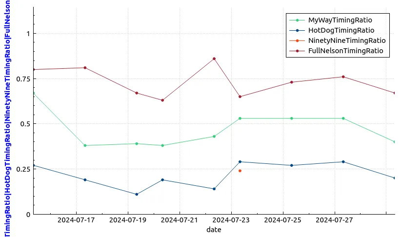
So what does this tell us? Now that this data has been normalized, we can confidently say these given songs will always appear in the following order, from earliest to latest in the concert:
- 9 Teen 90 Nine
- Hot Dog
- My Way
- Full Nelson
During this tour, fan interaction most often takes place in the later two thirds of the concert.
with spc as (
  select date, count(*) as songsPerConcert
  from performances_view
  where date >= "2024-07-16"
  group by date
)
select
  notes,
  songOrder,
  spc.songsPerConcert,
  round(cast(songOrder as float) / spc.songsPerConcert, 2) as timingRatio
from fan_performances
left join spc using (date)
where date >= "2024-07-16" order by date;
| notes | songOrder | songsPerConcert | timingRatio |
|---|---|---|---|
| (With fan Radio Contest Winner) | 7 | 16 | 0.44 |
| (With fan from crowd) | 13 | 16 | 0.81 |
| (Fans onstage) | 6 | 16 | 0.38 |
| (With Maxwell Narburgh (Fan from crowd)) | 10 | 16 | 0.63 |
| (Played this song with Fred in the crowd) | 5 | 14 | 0.36 |
| (George Michael cover)(Invited a fan “Blaze” up on stage) | 10 | 14 | 0.71 |
| (With a fan named Josh) | 11 | 17 | 0.65 |
| (Played “for Drake”, who was in the crowd, followed by crowd boos) | 14 | 17 | 0.82 |
| (Until second chorus; Fan request) | 15 | 17 | 0.88 |
| (Ministry cover)(Snippet - Wes playing main riff while Fred talked to crowd) | 16 | 17 | 0.94 |
| (All opening acts + some fans on stage) | 17 | 17 | 1.0 |
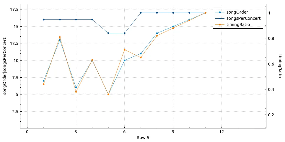
This information tells me that Hot Dog may not be a good choice of song to practice. It happens too early in the sets for fan interaction to take place compared to My Way. 9 Teen 90 Nine may still be a good choice due to how unlikely the song appears in the set.
Further questions
I could keep on going with this analysis forever. I could also revisit my previous assertions as more concerts occur in this tour, but it’s time for me to wrap up for now.
Some other questions I would like to ask:
- Are there any other songs that are performed in this tour during the sweet spot of fan interaction?
- Boiler may be a good candidate for this, in case we need to pick a new song.
- Will my findings for this concert remain consistent throughout the course of this tour?
- This is just a matter of running the same queries on updated data, meaning I need to run the scraper once in a while to do so.
Improvements
Overall, I’m happy with the improvements I made, and the information I learned from Limp Bizkit’s set list data. I’m also excited to be more confident with SQL, which will serve me well in my data analysis going forward!
There are some improvements I would like to make throughout various parts of my system, though:
- When scraping, I don’t save concerts into my database when there are no performances. I treat them as if they never happened, which has confused me multiple times when comparing my data with the data on setlist.fm.
- Here’s an example of a concert with no song data.
- I haven’t decided if I should save the concert in my database or ignore it.
- When running the scraper multiple times, I run the risk of encountering 429, or “Too many requests”, errors.
- Recording stats about the application, such as when I start encountering 429 errors and when I start scraping, can help me fine-tune when and how much I should scrape before running into those errors.
- Finding the start and end pages to scrape can be improved.
- I didn’t add any argument handling in my second iteration of my scraper. If I would like to automate some of this process, having these options would be helpful.
- Filtering my data by fan performances instead of fan interactions needs to improve.
- It was easier for me to add a new column to a table in a spreadsheet and add data to it than it was with SQL, so I put it off. This has made my data noisy, which does not help with my decision-making.
- I could either edit the data from the
notescolumn so my filters will pass, or add a new column called “FanPerformed”, or something similar - This also impacts my ability to determine if fans made a choice to play a specific song, or how many guest performers used a sign to grab the band’s attention. This was a big part of my research the first time around.
- Analyzing YouTube videos was monumentally useful, but took a lot of time. Is there a way I can incorporate that into my data ingress at all?
- Perhaps I can generate search queries using data from the
performances_viewtable, find a few video candidates, and then add whether a fan performed.
- Perhaps I can generate search queries using data from the
- Using SQLite was a nice way to quickly get started, but there were some functions I learned would be very useful that were lacking. Perhaps tools like MySQL or PostgreSQL can help make my queries easier to write.
Conclusion
I hope this article helped you learn some SQL! On top of that, I hope you learned some new things about some technologies that can help you do something similar.
This is my first dip into data analysis, which was very fun! I’m no superforecaster by any means, but we’ll see whether my analysis pays off. At the moment, My Way and 9 Teen 90 Nine still seem like good choices of songs to learn, while Hot Dog may not be a good choice, due to the fact it’s played earlier in the set. Our additional strategies, such as making our way to the stage about halfway through the show and making signs, will increase our chances of getting on stage.
That’s enough for now. Thanks for reading, and I’ll see you next time!